Starting with QubeSpec
First lets just quickly import some basic modules and QubeSpec. .. code:: ipython3
#importing modules import numpy as np import matplotlib.pyplot as plt; plt.ioff()
nan= float(‘nan’) pi= np.pi e= np.e
c= 3e8 h= 6.62*10**-34 k= 1.38*10**-23
%load_ext autoreload %autoreload 2
import QubeSpec as IFU import QubeSpec.Plotting as emplot import QubeSpec.Fitting as emfit import yaml
Initializing the QubeSpec and preparing the data for fitting
In order to make things easier for the user, I writen a simple dictionary called QubeSpec_setup. You can define all the necessary variables in this dictionary and then just run all the cells. Although there is a short description next to it, there will be full explanation of each variable accompanying the each function.
# Lets define additional info
PATH='/Users/jansen/My Drive/Astro/'

QubeSpec_setup = {}
######################
# Basic Properties
QubeSpec_setup['z'] = 6.851 # Redshift of the object
QubeSpec_setup['ID'] = 'COS30_R2700' # Name of the object
QubeSpec_setup['instrument'] = 'NIRSPEC_IFU_fl' # Name of the instrument - KMOS, SINFONI, NIRSPEC_IFU (when original units Fnu from pipeline), NIRSPEC_IFU_fl (for GTO pipeline Flambda)
QubeSpec_setup['band'] = 'R2700' # Or PRISM, doesnt matter for JWST - For KMOS and SINFONI it should H or K or HK or YJ or Hsin, Ksin for SINFONI
QubeSpec_setup['save_path'] = PATH+'COS30_IFS/Saves/' # Where to save all the info.
QubeSpec_setup['file'] = PATH+'COS30_IFS/Data/COS30-COS-6.80-S_jw1217_o007_ff_px0.05_drizzle_ODfde95.0_VSC_MRC_MSA_EMSA_m2ff_xyspikes96_CTX1068.pmap_v1.8.2_g395h-f290lp_cgs_s3d.fits'# Path to the Data Cube
QubeSpec_setup['norm'] = 1e-15 # Normalization to make the integrated spectrum around 0.5-8

#####################
# PSF Matching info
QubeSpec_setup['PSF_match'] = True
QubeSpec_setup['PSF_match_wv'] = 5.2

#####################
# Masking Channels
QubeSpec_setup['mask_threshold'] = 6 # multiple of the median error to mask
QubeSpec_setup['mask_channels'] = []  # any particular channels to mask - with JWST not necessarily

#####################
# Background Subtraction
QubeSpec_setup['Source_mask'] = PATH+'COS30_IFS/Data/R2700_source.fits' # path to find the source mask to mask the source during background subtraction - Can be None but then you have to supply wavelength range around some emission line to construct a line map and let sextractor create the mask
QubeSpec_setup['line_map_wavelength'] = [3.92,3.94] # Wavelength range used to create a line map for source detection - only used if 'Source_mask' is None

#####################
# Extracting spectrum
QubeSpec_setup['Object_center'] = [59,50] # X,Y - center of the object
QubeSpec_setup['Aperture_extraction'] = 0.2 # radius of the aperture to extract the the 1D spectrum
# Error stuff - explained below
QubeSpec_setup['err_range']=[3.95,4.05, 5,5.1] # err ranges for renormalising the error extension
QubeSpec_setup['err_boundary'] = 4.1 # where to switch - location of the detector gap

#####################
# Fitting Spaxel by Spaxel
QubeSpec_setup['Spaxel_mask'] = PATH+'COS30_IFS/Data/R2700_source_mask.fits' # which spaxel to fit in spaxel-by-spaxel fitting - source mask and Spaxel mask can be the same
QubeSpec_setup['ncpu'] = 8 # number of cores to use for
QubeSpec_setup['Spaxel_Binning'] = 'Nearest' # What binning option to use  - 'Nearest', 'Single'


with open(QubeSpec_setup['save_path']+'QubeSpec_setup.yml', 'w') as outfile:
    yaml.dump(QubeSpec_setup, outfile, default_flow_style=False, allow_unicode=True)
Initalize the cube
Here we initialize the Cube class and load the cube. We also perform few minor preps. You will need:
Full_path = path to the fits cube
z - redshift of the source
ID - name of the source. For example: COS-3018_R2700
flag - Instrument glag - Options: ‘KMOS’, ‘SINFONI’, ‘NIRSPEC’, ‘NIRSPEC_fl’ and ‘MIRI’
savepath - When do you save all of the products.
Band - For flag - ‘NIRSPEC’ or ‘NIRSPEC_fl’ just go ‘NIRSPEC’ , ‘KMOS’: ‘YJ’, ‘H’, ‘K’; ‘SINFONI’: ‘Ysin’, ‘Hsin’, ‘Ksin’
norm - normalization of the cube to make the integrated spectrum ~0.5-5 ish. The code just handles things better when the spectra are around 1.
Cube = IFU.Cube( Full_path = QubeSpec_setup['file'],\
                z =  QubeSpec_setup['z'], \
                ID =  QubeSpec_setup['ID'] ,\
                flag =  QubeSpec_setup['instrument'] ,\
                savepath = QubeSpec_setup['save_path'] ,\
                Band = 'NIRSPEC',\
                norm = QubeSpec_setup['norm'])
Masking
Here we are going to mask some of the obvious outliers. In JWST data, they have often obvious spikes in the error extension. The code caluclates the median error value and then masks any pixels that are higher than mask_threshold* this meadian. We can also give a list of indices representing channels that need some manual masking. The recommended mask_threshold value of 6
Cube.mask_JWST(0, threshold= QubeSpec_setup['mask_threshold'], spe_ma=QubeSpec_setup['mask_channels'])
Background Subtraction
When dealing with JWST data, it is important to perform the background subtraction. This algorithm is courtesy of Francesco D’Eugenio. The code estimates the median background in each channel, masking out any pixels that are not covered by the cube (the edges) and the source - see later. The Median background is estimate across filter_size (default 5,5, but can be changed). Once the background cube is estimated, it is smoothened by a median filter (with wave_smooth =25 channels, another free parameter).
There are currently two ways of dealing with the source mask:
You supply the actual source mask from QFits view.
You let the code find the object using the source etxractor. At that point, please supply the wave_range =[X,Y], which will be used to collapse the cube to create a line map. Furthermore, you can change the detection_threshold=3 for the sextractor.
Eitherway, at the end you will get a background (Cube.background) and a subtracted flux cube (Cube.flux)
if any(QubeSpec_setup['Source_mask']) !=None:
    print('Loading source mask from file')
    source_bkg = IFU.sp.QFitsview_mask(QubeSpec_setup['Source_mask']) # Loading background mask
Cube.background_subtraction( source_mask=source_bkg,\
 wave_range=QubeSpec_setup['line_map_wavelength'],\
  plot=1) # Doing background subtraction

plt.show()
Cube.PSF_matching(PSF_match = QubeSpec_setup['PSF_match'],\
                    wv_ref= QubeSpec_setup['PSF_match_wv'])
Extracting your first spectrum
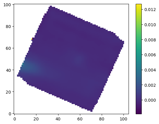
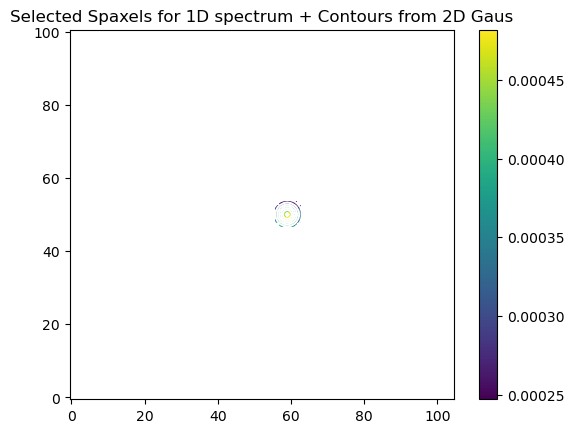
In order to extract a specturm we first collpase the cube into a white light image using collpase_white function. Then we find the center of the galaxy from the continuum. With KMOS or seeing limited SINFONI observations, we could use 2D Gaussian in order to find the center of an object. With NIRSpec and SINFONI AO, galaxies can be quite clumy and hence it often fails. Therefore I would suggest using the manual= [x,y] keyword in order to define it yourself.
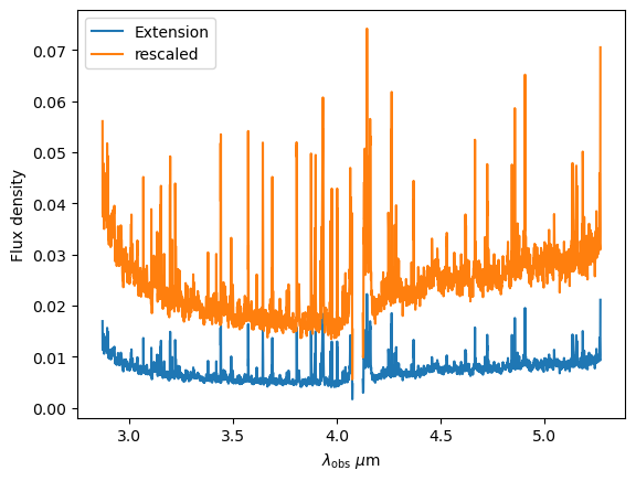
Next we select and collapse the aperture using the D1_spectra_collapse with he following keywords: 1) radius of the extraction circle (units of arcseconds) 2) add_save = string - name appended to the basic file name when saving the spectrum 3) err_range - list of 2 or 4 numbers. This are wavelength boundries used (read full explanation below) 4) boundary - if you use 4 numbers in err_range, boundary will be where the error calc will be split. 5) plot_err = 1/0 - do you want to plot the comparison of the errors estimated in this code and the ones from the NIRSpec extension
For NIRSpec spectra: Unfortunately, we cannot use the error extension from the pipeline as there is scaling issue at hand. However, the error extension maintains all of the correlation between channels. Because of that, we estimate the error from the error extension and then compared to the median value of this error array to the standard deviation of the continuum. The err_range values are defining the wavelength region that is used to estimate the standard deviation of the spectrum. There are two options of supplying the right info:
err_range = [lower, upper] - in this case yo the upper and lower wavelength range of emission line free part of the spectrum. The code will estimate the standard deviation of that part to the error extension and scale it.
err_range = [lower_a, upper_a, lower_b, upper_b] and boundary=4.1 - in this case yo the upper and lower wavelength range of TWO seperate emission line free sections of the spectrum. The code will estimate the standard deviation of that part to the error extension and scale it for each section. The boundary value is the wavelength value where you apply the the lower or upper scaling factor. Example below:
err_range=[3.95,4.05, 5,5.1] and boundary=4.1
The code will estimate the standard deviation from the spectrum and hence the scaling factor for two section: 3.95-4.05 and 5.-5.1. It will then applying the two scaling factor to error extension with lambda<4.1 and lambda>4.1.
So the err_range should be section of spectra without any emission lines. The boundary should be somewhere between emission lines of interest of in case of R2700 - the detector gap
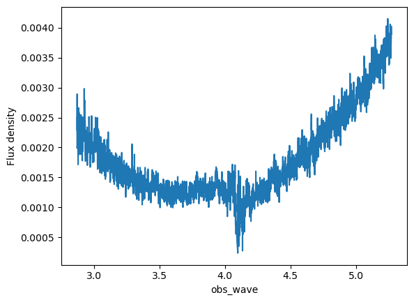
Cube.collapse_white(1)

Cube.find_center(1, manual=QubeSpec_setup['Object_center'])
Cube.D1_spectra_collapse(1, addsave='',rad=QubeSpec_setup['Aperture_extraction'],\
 err_range=QubeSpec_setup['err_range'],\
  boundary=QubeSpec_setup['err_boundary'],\
   plot_err=1)
plt.show()

Saving the class and resume
At any point you can save the Cube class with save(file_path) function. Later on you can Initialize the empty class again and then load it with load(file_path)
Cube.save('/Users/jansen/Test.txt') #

Cube2 = IFU.Cube()
Cube2.load('/Users/jansen/Test.txt')
Plotting spectrum
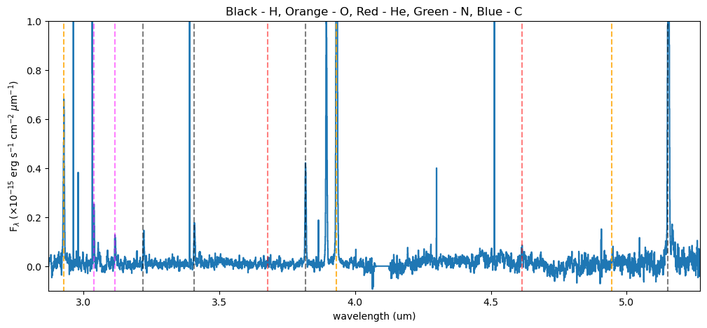
Lets just have a look at all the emission lines in the spectrum.
f, ax = plt.subplots(1, figsize=(12,5))

ax.plot(Cube.obs_wave, Cube.D1_spectrum, drawstyle='steps-mid')

ylow = -0.2
yhig = 10

ax.vlines(0.5008*(1+Cube.z),ylow,yhig, linestyle='dashed',color='orange', alpha=0.8)
ax.vlines(0.3727*(1+Cube.z),ylow,yhig, linestyle='dashed',color='orange', alpha=0.8)
ax.vlines(0.6300*(1+Cube.z),ylow,yhig, linestyle='dashed',color='orange', alpha=0.8)


ax.vlines(0.6563*(1+Cube.z),ylow,yhig, linestyle='dashed',color='k', alpha=0.5)
ax.vlines(0.4861*(1+Cube.z),ylow,yhig, linestyle='dashed',color='k', alpha=0.5)
ax.vlines(0.4340*(1+Cube.z),ylow,yhig, linestyle='dashed',color='k', alpha=0.5)
ax.vlines(0.4100*(1+Cube.z),ylow,yhig, linestyle='dashed',color='k', alpha=0.5)
ax.vlines(0.1215*(1+Cube.z),ylow,yhig, linestyle='dashed',color='k', alpha=0.5)
ax.vlines(0.6731*(1+Cube.z),ylow,yhig, linestyle='dashed',color='k', alpha=0.5)

ax.vlines(0.3869*(1+Cube.z),ylow,yhig, linestyle='dashed',color='magenta', alpha=0.5)
ax.vlines(0.3968*(1+Cube.z),ylow,yhig, linestyle='dashed',color='magenta', alpha=0.5)
ax.vlines(0.2424*(1+Cube.z),ylow,yhig, linestyle='dashed',color='magenta', alpha=0.5)


ax.vlines(0.4686*(1+Cube.z),ylow,yhig, linestyle='dashed',color='red', alpha=0.5)
ax.vlines(0.5877*(1+Cube.z),ylow,yhig, linestyle='dashed',color='red', alpha=0.5)

ax.set_title('Black - H, Orange - O, Red - He, Green - N, Blue - C')

ax.set_xlabel('wavelength (um)')
ax.set_ylabel(r'F$_\lambda$ ($\times 10^{-15}$ erg s$^{-1}$ cm$^{-2}$ $\mu$m$^{-1}$)')

ax.set_xlim(min(Cube.obs_wave), max(Cube.obs_wave))
ax.set_ylim(-0.1, 1)
plt.show()
After these steps, the Cube instance should have the following attributes:
Cube.flux- Flux data cubeCube.error_cube- Error data cubeCube.obs_wave- observed wavelengthCube.D1_spectrum- Collapsed 1D spectrumCube.D1_spectrum_er- error on the collapsed 1D spectrumCube.Median_stack_white- continuum imageCube.header- Header of the data cube from the fits fileCube.save_path- path where we are saving stuff