Fitting a single spectrum
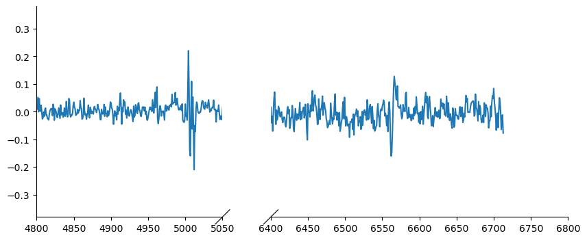
In this section we will fit the extracted spectrum from the previous section. First we will quickly import some modules.
#importing modules
import numpy as np
import matplotlib.pyplot as plt; plt.ioff()

c= 3e8

import QubeSpec as IFU
import QubeSpec.Plotting as emplot
import QubeSpec.Fitting as emfit
import yaml
Core Fitting module
At first we will look into the Fitting class, how it works, what results it generates and how can we calculate other quantities. Then I will introduce the wrapper function I wrote in order to speed up things when fitting.
First lets initalize the Fitting class:
- class QubeSpec.Fitting.Fitting(wave='', flux='', error='', z='', N=5000, ncpu=1, progress=True, priors={'z': [0, 'normal_hat', 0, 0.003, 0, 0]})
Simple class containing everything that we need to fit a spectrum and also all of its results.
- Parameters:
wave (array) – observed wavelength in microns
flux (array) – flux of the spectrum
error (array) – error on the spectrum
z (float) – redshift of the source
N (int - optional) – number of points in the chain - default 5000
ncpu (int - optional) – number of cpus used to fit - I find that the overheads can be bigger what using multipleprocessing then the speed up. Experiment or keep to 1
progress (bool - optional) – progress bar for the emcee bit
priors (dict - optional) – dictionary with all of the priors to update
- fitting_Halpha(model='gal')
Method to fit Halpha+[NII +[SII]]
- Parameters:
str (model -) –
current valid models names and their variable names/also prior names:
gal - ‘z’, ‘cont’,’cont_grad’, ‘Hal_peak’, ‘NII_peak’, ‘Nar_fwhm’, ‘SIIr_peak’, ‘SIIb_peak’
outflow - ‘z’, ‘cont’,’cont_grad’, ‘Hal_peak’, ‘NII_peak’, ‘Nar_fwhm’, ‘SIIr_peak’, ‘SIIb_peak’, ‘Hal_out_peak’, ‘NII_out_peak’, ‘outflow_fwhm’, ‘outflow_vel’
BLR_simple - ‘z’, ‘cont’,’cont_grad’, ‘Hal_peak’,’BLR_Hal_peak’, ‘NII_peak’, ‘Nar_fwhm’, ‘BLR_fwhm’, ‘zBLR’, ‘SIIr_peak’, ‘SIIb_peak’
BLR - ‘z’, ‘cont’,’cont_grad’, ‘Hal_peak’,’BLR_Hal_peak’, ‘NII_peak’, ‘Nar_fwhm’, ‘BLR_fwhm’, ‘zBLR’, ‘SIIr_peak’, ‘SIIb_peak’
- QSO_BKPL - ‘z’, ‘cont’,’cont_grad’, ‘Hal_peak’, ‘NII_peak’, ‘Nar_fwhm’,
’Hal_out_peak’, ‘NII_out_peak’, ‘outflow_fwhm’, ‘outflow_vel’, ‘BLR_Hal_peak’, ‘zBLR’, ‘BLR_alp1’, ‘BLR_alp2’, ‘BLR_sig’
- fitting_Halpha_OIII(model, template=0)
Method to fit Halpha + [OIII] + Hbeta+ [NII] + [SII]
- Parameters:
str (model -) –
current valid models names and their variable names/also prior names:
gal - ‘z’, ‘cont’,’cont_grad’, ‘Hal_peak’, ‘NII_peak’, ‘Nar_fwhm’, ‘SIIr_peak’, ‘SIIb_peak’, ‘OIII_peak’, ‘Hbeta_peak’
outflow - ‘z’, ‘cont’,’cont_grad’, ‘Hal_peak’, ‘NII_peak’,’OIII_peak’, ‘Hbeta_peak’,’SIIr_peak’, ‘SIIb_peak’,’Nar_fwhm’, ‘outflow_fwhm’, ‘outflow_vel’, ‘Hal_out_peak’,’NII_out_peak’, ‘OIII_out_peak’, ‘Hbeta_out_peak’
BLR - ‘z’, ‘cont’,’cont_grad’, ‘Hal_peak’, ‘NII_peak’,’OIII_peak’, ‘Hbeta_peak’,’SIIr_peak’, ‘SIIb_peak’, ‘Nar_fwhm’, ‘outflow_fwhm’, ‘outflow_vel’, ‘Hal_out_peak’,’NII_out_peak’, ‘OIII_out_peak’, ‘Hbeta_out_peak’ , ‘BLR_fwhm’, ‘zBLR’, ‘BLR_Hal_peak’, ‘BLR_Hbeta_peak’
BLR_simple - ‘z’, ‘cont’,’cont_grad’, ‘Hal_peak’, ‘NII_peak’,’OIII_peak’, ‘Hbeta_peak’,’SIIr_peak’, ‘SIIb_peak’, ‘Nar_fwhm’, ‘BLR_fwhm’, ‘zBLR’, ‘BLR_Hal_peak’, ‘BLR_Hbeta_peak’
- fitting_OIII(model, Fe_template=0, plot=0)
Method to fit [OIII] + Hbeta
- Parameters:
str (template -) –
current valid models names and their variable names/also prior names:
gal - ‘z’, ‘cont’,’cont_grad’, ‘OIII_peak’, ‘Nar_fwhm’, ‘Hbeta_peak’ - Hbeta and [OIII] kinematics are linked together
outflow - ‘z’, ‘cont’,’cont_grad’, ‘OIII_peak’, ‘OIII_out_peak’, ‘Nar_fwhm’, ‘outflow_fwhm’, ‘outflow_vel’, ‘Hbeta_peak’, ‘Hbeta_out_peak’ - Hbeta and [OIII] kinematics are linked together
str – name of the FeII template you want to fit - Tsuzuki, BG92, Veron
- fitting_general(fitted_model, labels, logprior=None, nwalkers=64, skip_check=False)
Fitting any general function that you pass. You need to put in fitted_model, labels and you can pass logprior function or number of walkers.
- Parameters:
fitted_model (callable) – Function to fit
labels (list) – list of the name of the paramters in the same order as in the fitted_function
priors (dict - optional) – dictionary with all of the priors to update
logprior (callable function) – logprior evaluation function - use emfit.logprior_general or emfit.logprior_general_scipy
nwalkers (int - optional) – default 64 walkers for the MCMC
The priors variable should be in a form of a dictionary like:
‘name of the variable’ - I will give a full list of variable for each models below.
intial value - inital value for the fit - if you want the code to decide put 0
‘shape of the prior’ - ‘uniform’, ‘loguniform’ (uniform in logspace), ‘normal’, ‘normal_hat’ (truncated normal distribution)
once this is initialized, we can use some of the prewritten models or use a custom function fitting. Setting up a custom function fitting is a little bit more complex,
but once understood, it is in no way complicated or long. In order fit a custom function you need to use the Fitting.fitting_general method of the Fitting class.
Fitting Custom Function
Once we initialize the Fitting class we need to define couple of things:
calllable function with variable:
wavelength,z(redshift) and rest of the free parameters and it will return a 1D array of flux values.name of the parameters in a list -
labelsprior dictionary with initial values -
priors
Below I will show an example of such function that fits a spectrum from [OII] to [SII] with one Gaussian component with tied kinematics plus a continuum described as power law.
def gauss(x, k, mu,FWHM):
    sig = FWHM/3e5*mu/2.35482
    expo= -((x-mu)**2)/(2*sig*sig)

    y= k* e**expo

    return y
from astropy.modeling.powerlaws import PowerLaw1D

def Full_optical(x, z, cont,cont_grad,  Hal_peak, NII_peak, OIIIn_peak, Hbeta_peak, Hgamma_peak, Hdelta_peak, NeIII_peak, OII_peak, OII_rat,OIIIc_peak, HeI_peak,HeII_peak, Nar_fwhm):
    # Halpha side of things
    Hal_nar = gauss(x, Hal_peak, 6564.52*(1+z)/1e4, Nar_fwhm)
    NII_nar_r = gauss(x, NII_peak, 6585.27*(1+z)/1e4, Nar_fwhm)
    NII_nar_b = gauss(x, NII_peak/3, 6549.86*(1+z)/1e4, Nar_fwhm)

    Hgamma_nar = gauss(x, Hgamma_peak, 4341.647191*(1+z)/1e4, Nar_fwhm)
    Hdelta_nar = gauss(x, Hdelta_peak, 4102.859855*(1+z)/1e4, Nar_fwhm)


    # [OIII] side of things

    OIII_nar = gauss(x, OIIIn_peak, 5008.24*(1+z)/1e4, Nar_fwhm) + gauss(x, OIIIn_peak/3, 4960.3*(1+z)/1e4, Nar_fwhm)
    Hbeta_nar = gauss(x, Hbeta_peak, 4862.6*(1+z)/1e4, Nar_fwhm)

    NeIII = gauss(x, NeIII_peak, 3869.68*(1+z)/1e4, Nar_fwhm ) + gauss(x, 0.322*NeIII_peak, 3968.68*(1+z)/1e4, Nar_fwhm)

    OII = gauss(x, OII_peak, 3727.1*(1+z)/1e4, Nar_fwhm )  + gauss(x, OII_rat*OII_peak, 3729.875*(1+z)/1e4, Nar_fwhm)

    OIIIc = gauss(x, OIIIc_peak, 4364.436*(1+z)/1e4, Nar_fwhm )
    HeI = gauss(x, HeI_peak, 3889.73*(1+z)/1e4, Nar_fwhm )
    HeII = gauss(x, HeII_peak, 4686.0*(1+z)/1e4, Nar_fwhm )

    contm = PowerLaw1D.evaluate(x, cont,6564.52*(1+z)/1e4, alpha=cont_grad)

    return contm+Hal_nar+NII_nar_r+NII_nar_b + OIII_nar + Hbeta_nar + Hgamma_nar + Hdelta_nar + NeIII+ OII + OIIIc+ HeI+HeII

# list of variable in the right order as in the function above.
labels= ['z', 'cont','cont_grad',  'Hal_peak', 'NII_peak', 'OIII_peak', 'Hbeta_peak','Hgamma_peak', 'Hdelta_peak','NeIII_peak','OII_peak','OII_rat','OIIIaur_peak', 'HeI_peak','HeII_peak', 'Nar_fwhm']


z = 6.4
dvmax = 1000/3e5*(1+z)
dvstd = 200/3e5*(1+z)

priors={'z':[z,'normal_hat', z, dvstd, z-dvmax, z+dvmax]}
priors['cont']=[0.1,'loguniform', -3,1]
priors['cont_grad']=[0.2,'normal', 0,0.2]
priors['Hal_peak']=[5.,'loguniform', -3,1]
priors['NII_peak']=[0.4,'loguniform', -3,1]
priors['Nar_fwhm']=[300,'uniform', 200,900]
priors['OIII_peak']=[6.,'loguniform', -3,1]
priors['OI_peak']=[1.,'loguniform', -3,1]
priors['HeI_peak']=[1.,'loguniform', -3,1]
priors['HeII_peak']=[1.,'loguniform', -3,1]
priors['Hbeta_peak']=[2,'loguniform', -3,1]
priors['Hgamma_peak'] = [1.,'loguniform',-3,1]
priors['Hdelta_peak'] = [0.5,'loguniform',-3,1]
priors['NeIII_peak'] = [0.3,'loguniform',-3,1]
priors['OII_peak'] = [0.4,'loguniform',-3,1]
priors['OII_rat']=[1,'normal_hat',1,0.2, 0.2,4]
priors['OIIIaur_peak']=[0.2,'loguniform', -3,1]
Then we can initialize the Fitting class as variable optical and then run it in the following manner:
if __name__ == '__main__':
    optical = emfit.Fitting(obs_wave, flux, error, z, priors=priors, N=5000, ncpu=3)
    optical.fitting_general( Full_optical, labels)
Getting useful info out of the fit:
Regardless of method we use to fit the spectrum, the Fitting as optical class should now have few attributes with all of the results that we need:
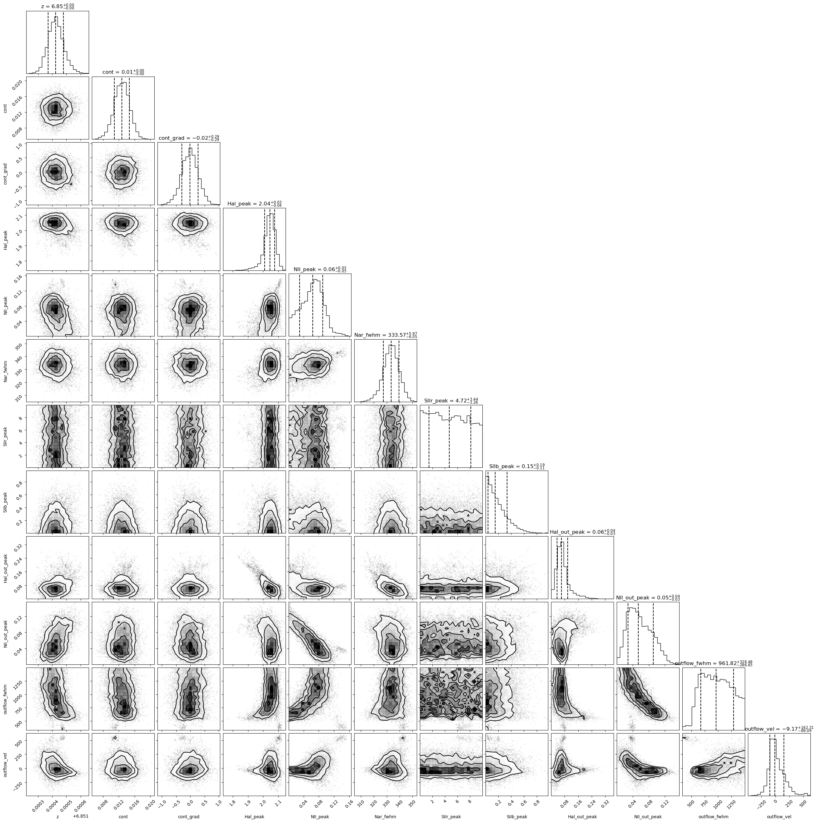
optical.fitted_model- returns model/function that was used to fit the spectrumoptical.yeval- return evaluated best fitted modeloptical.chains- return dictionary with burned it chains - each variable has an array with all of the chain values (the names are either supplied by user as labels or are described by each of the fitting functions)optical.like_chains- return likelihod evaluation for each of the chain valueoptical.props- return a dictionary containing each variable (median) and the 68% confidence interval. It also contains an array of best fit parametersoptical.props['popt']that can be directly used to evaluate thefitted_modeloptical.BIC,optical.chi2- BIC and chi2 value of the fitoptical.wave- wavelength used for the fitoptical.flux- flux used for the fitoptical.error- error on flux used for the fitoptical.corner()- method - plots a corner plot
In order to calculate integrated fluxes of each emission line we can use the IFU.sp.flux_calc_mcmc() with the following:
- sp.flux_calc_mcmc(mode, norm=1, N=2000, wv_cent=5008, peak_name='', fwhm_name='', ratio_name='')
Calculates flux and 68% confidence iterval.
- Parameters:
object (fit_obj -) – Fitting class object
string (ratio_name -) – modes: general, OIIIn, OIIIw, OIIIt, Han, NII, Hbeta, SIIr, SIIb
value (norm -) – normalization used in the QubeSpec cube class
int (N -) – number of sampling of the chains
float (wv_cent -) – rest-frame wavelength in ang of the line if mode=’general’
string – if mode=’general’ name of the peak name to use
string – if mode=’general’ name of the fwhm name to use
string – if mode=’general’ name of the ratio to use (e.g. in [OII])
- Return type:
array of median value and +- 1sigma
Examples:
print('[OIII] flux from custom', IFU.sp.flux_calc_mcmc(optical, 'general', Cube.flux_norm, wv_cent=5008, peak_name='OIII_peak', fwhm_name='Nar_fwhm' ))
print('[OII]3727 flux from custom',IFU.sp.flux_calc_mcmc(optical, 'general', Cube.flux_norm, wv_cent=3727, peak_name='OII_peak', fwhm_name='Nar_fwhm', ratio_name='' ))
print('[OII]3729 flux from custom',IFU.sp.flux_calc_mcmc(optical, 'general', Cube.flux_norm, wv_cent=3729, peak_name='OII_peak', fwhm_name='Nar_fwhm', ratio_name='OII_rat' ))
Finally we can also save the results of the fitting like this:
optical.save(path)
and then load the results as:
Fitting 1D collpased spectrum from a cube.
now lets load the Cube object from previous page.
Cube = IFU.Cube()
Cube.load('/Users/jansen/Test.txt')
The main The QubeSpec class contains few methods that are designed to fit the collapsed 1D spectra that were extracted in the previous section. The next few sub sections will describe them and show them in action. All of the functions
Fitting Halpha only
models - Single_only, Outflow_only, BLR_only, BLR, Outflow, QSO_BKPL
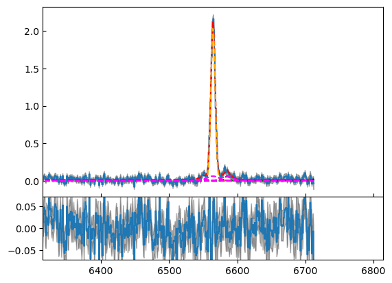
Cube.fitting_collapse_Halpha(models='Outflow') # priors=priors
plt.show()
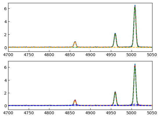
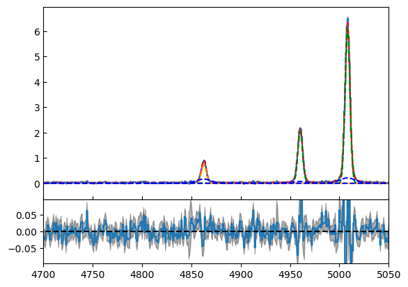
Fitting [OIII]
simple = 0 or 1 when 1, we tie the Hbeta and OIII kinematics together. Please just use simple = 1 - Unless fitting high luminosity AGN and when you get a decent fit the Hbeta still looks wonky.
models - Single_only, Outflow_only, BLR_only, BLR, Outflow, QSO_BKPL
which changes if you fit a single model.
# B14 style
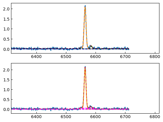
Cube.fitting_collapse_OIII(models='Outflow',simple=1, plot=1)
plt.show()

Fitting Halpha + [OIII]
models - Single_only, Outflow_only, BLR, QSO_BKPL, BLR_simple
Cube.fitting_collapse_Halpha_OIII(models='Outflow_only', plot=1)

plt.show()
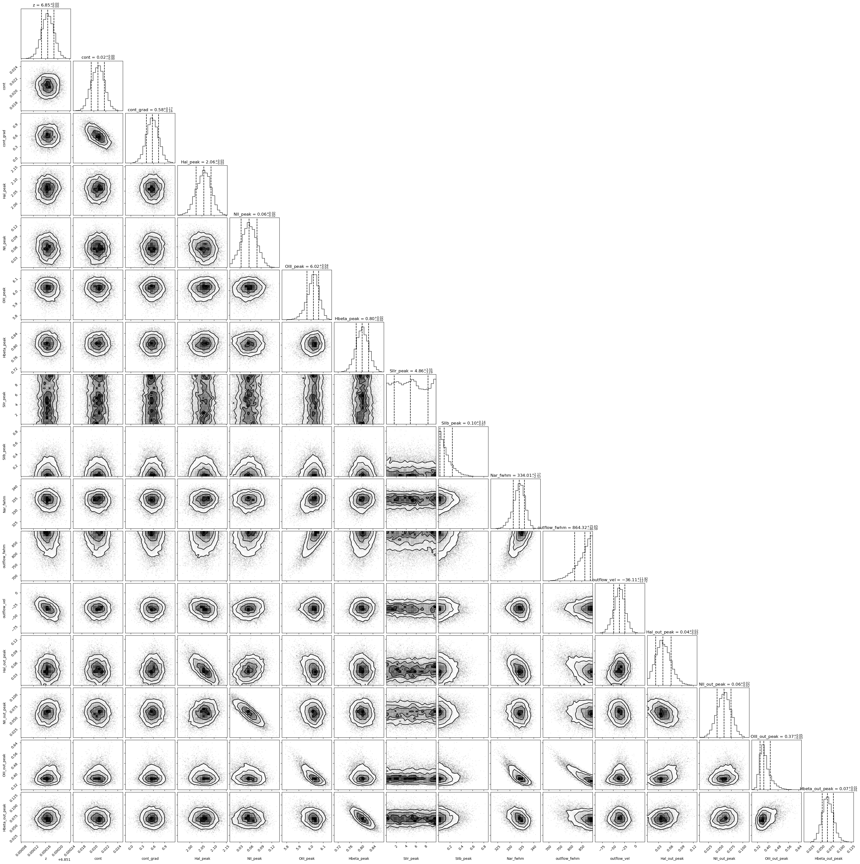
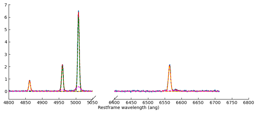
Cube.D1_fit_results
Fitting a custom model by passing a dictionary of components
Very highly experimental, still under development, use at your risk!
dvmax = 1000/3e5*(1+Cube.z)
dvstd = 200/3e5*(1+Cube.z)

model_inputs = {}
model_inputs["m_z"] = [Cube.z, ['normal_hat', Cube.z, dvstd, Cube.z-dvmax, Cube.z+dvmax]]
model_inputs["m_fwhm_nr"] = [400, ['uniform' , 100, 900]]
model_inputs["m_ContSlope"] = [0.001, ['normal', 0, 1]]
model_inputs["m_ContNorm"] = [0.1, ['loguniform', -3, 1]]

#model_inputs["m_fwhm_br"] = [700, ['uniform', 400, 1200]]

model_inputs["l_nr_Ha_peak"]= [1, ['loguniform', -3, 1]]
model_inputs["l_nr_Ha_wav"] = [0.656452255]

model_inputs["l_nr_Hb_peak"]= [1, ['loguniform', -3, 1]]
model_inputs["l_nr_Hb_wav"] = [0.4861]

model_inputs["l_nr_Hg_peak"]= [1, ['loguniform', -3, 1]]
model_inputs["l_nr_Hg_wav"] = [0.4341647191]

model_inputs["l_nr_Hd_peak"]= [1, ['loguniform', -3, 1]]
model_inputs["l_nr_Hd_wav"] = [0.410285985]

model_inputs["l_nr_HeI_peak"]= [1, ['loguniform', -3, 1]]
model_inputs["l_nr_HeI_wav"] = [0.388973]

model_inputs["l_nr_OIIIc_peak"]= [1,['loguniform', -3, 1]]
model_inputs["l_nr_OIIIc_wav"] = [0.43640436]

model_inputs["d_nr_NeIII_wav1"] = [0.386968]
model_inputs["d_nr_NeIII_wav2"] = [0.396868]
model_inputs["d_nr_NeIII_peak1"] = [1.0,['loguniform', -3, 1]]
model_inputs["d_nr_NeIII_ratio"] = [3.1055]

model_inputs["d_nr_NII_wav1"] = [0.6585273]
model_inputs["d_nr_NII_wav2"] = [0.654986]
model_inputs["d_nr_NII_peak1"] = [0.1,['loguniform', -3, 1]]
model_inputs["d_nr_NII_ratio"] = [3]

model_inputs["d_nr_OIII_wav1"] = [0.5008]
model_inputs["d_nr_OIII_wav2"] = [0.4960]
model_inputs["d_nr_OIII_peak1"] = [1,['loguniform', -3,1]]
model_inputs["d_nr_OIII_ratio"] = [2.99]

model_inputs["d_nr_OII_wav1"] = [0.3727]
model_inputs["d_nr_OII_wav2"] = [0.3729]
model_inputs["d_nr_OII_peak1"] = [0.9,['loguniform', -3, 1]]
model_inputs["d_nr_OII_ratio"] = [1,['uniform',0.2, 4]]


if __name__ == '__main__':
    optical_cus = emfit.Fitting(Cube.obs_wave, Cube.D1_spectrum, Cube.D1_spectrum_er,Cube.z, priors=priors, N=5000, ncpu=1) # Cube.obs_wave[use], Cube.D1_spectrum[use], Cube.D1_spectrum_er[use]
    optical_cus.fitting_custom(model_inputs, model_name='test')
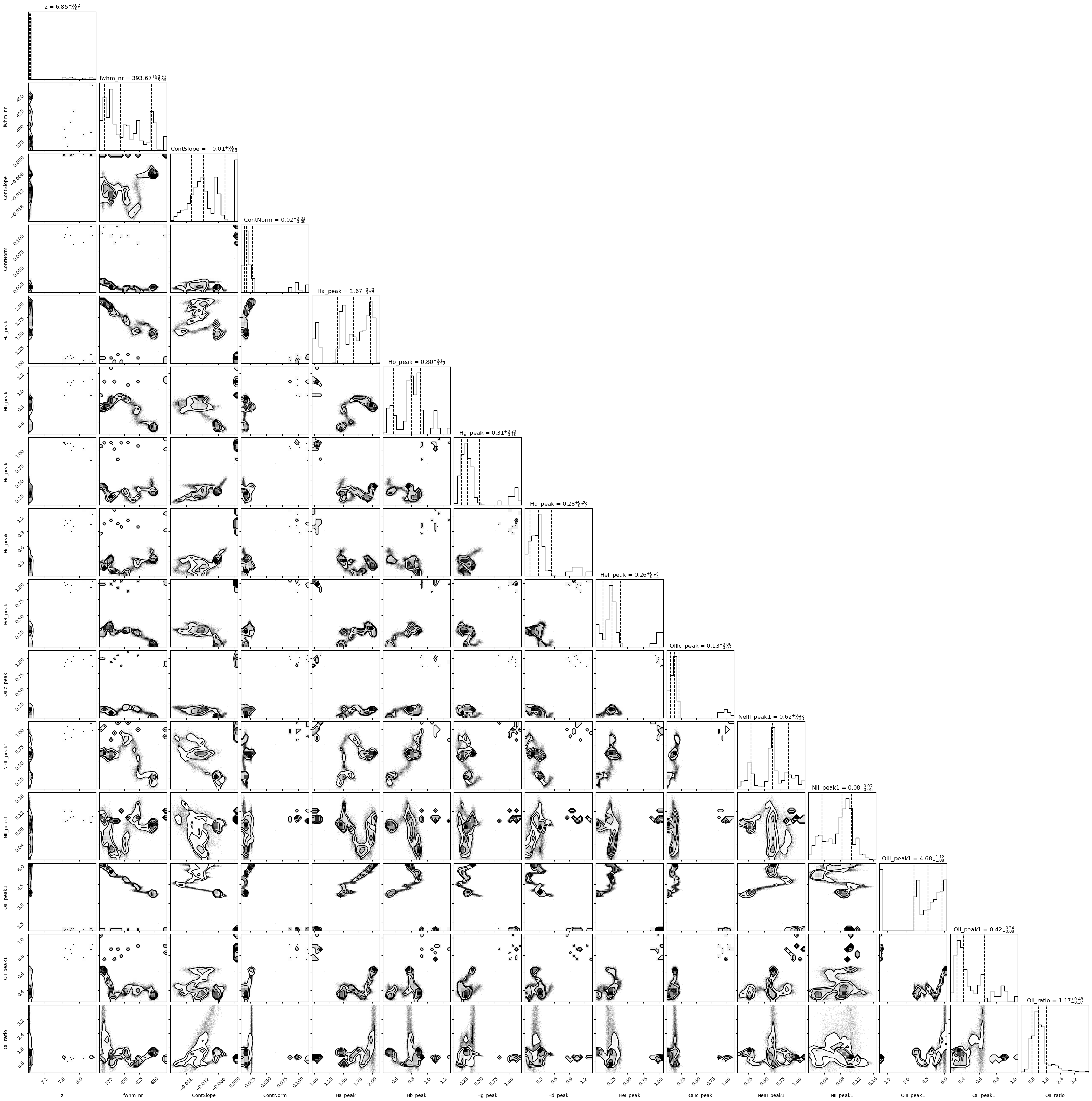
import corner

fig = corner.corner(
            IFU.sp.unwrap_chain(optical_cus.chains),
            labels = optical_cus.labels,
            quantiles=[0.16, 0.5, 0.84],
            show_titles=True,
            title_kwargs={"fontsize": 12})
#fig.savefig('~/corner_full.pdf')
plt.show()